Summary
I present here the additional material required to reproduce the figures included in the review entitled "Spatially-Resolved Spectroscopic Properties of Low-Redshift Star-Forming Galaxies", to be published in the Annual Review of Astronomy and Astrophysics.
In that review I report on the spatially-resolved spectroscopic properties of low-redshift star- forming galaxies (and their retired counter-parts), using results from the most recent Integral Field Spectroscopy galaxy surveys:
This compilation used publically available data, all processed using Pipe3D, to homogenize the results. Most of the datapructs are indeed publically avaiable:
However, to facilitate the replication of the figures and future comparisons I include here the processed files, just prepared to reproduce the trends observed and described in the review.Additional Material
The additional material included in this page comprises:
From this table it is created Figure 20 of the manuscript:
For Figures 1-8 and Fig. 10, those files corresponds to 2D maps comprising: (1) the density distributions shown in different figures along the article (tracing the main reported trends between parameters; and (2) the EW(Ha) at each location within the reported distributions. The 2D distributions are stored in fits that include in the header the WCS required to determine at which location in each diagram correspond each pixel.
| Figure 1: BPT diagram for the integrated properties | |
|---|---|
| Density maps: NN_den_plBPT_mass_den.fits (contours) | |
| EW maps: NN_EW_plBPT_mass_den.fits (colormaps) | |
| Access to the fitsfiles to generate this figure | |
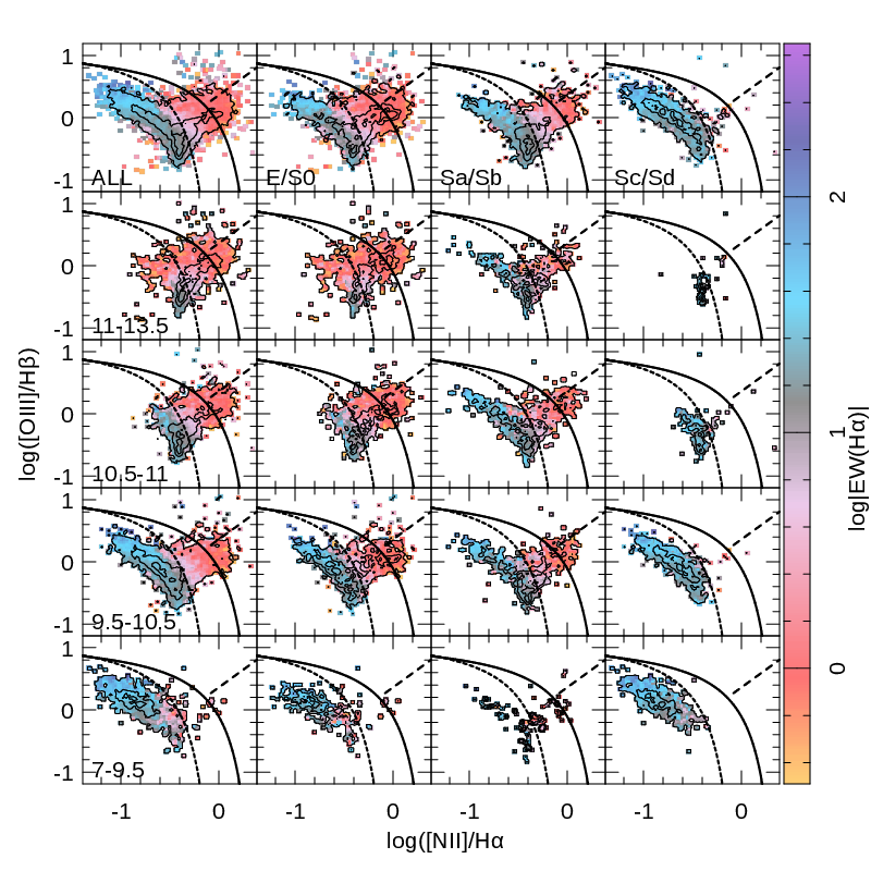 |
NN order in Figure: 01 02 03 04 17 18 19 20 13 14 15 16 09 10 11 12 05 06 07 08
|
| Figure 2: SFR-M* distribution | |
|---|---|
| Density maps: NN_den_plSFMS.fits (contours) | |
| EW maps: NN_EW_plSFMS.fits (colormaps) | |
| Access to the fitsfiles to generate this figure | |
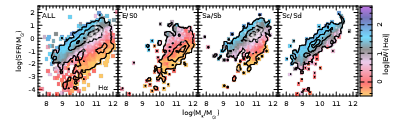 |
NN order in Figure:
01 02 03 04 |
| NOTE: For the SFR_SSP (Sanchez et al. 2018), use: 05 06 07 08 | |
| Figure 3: M-O/H distribution using the t2 calibrator | |
|---|---|
| Density maps: NN_den_plM_OH.fits (contours) | |
| EW maps: NN_EW_plM_OH.fits (colormaps) | |
| Access to the fitsfiles to generate this figure | |
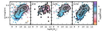 |
NN order in Figure:
01 02 03 04 |
| NOTE: For O/H using the pyqz calibrator, use: 05 06 07 08 | |
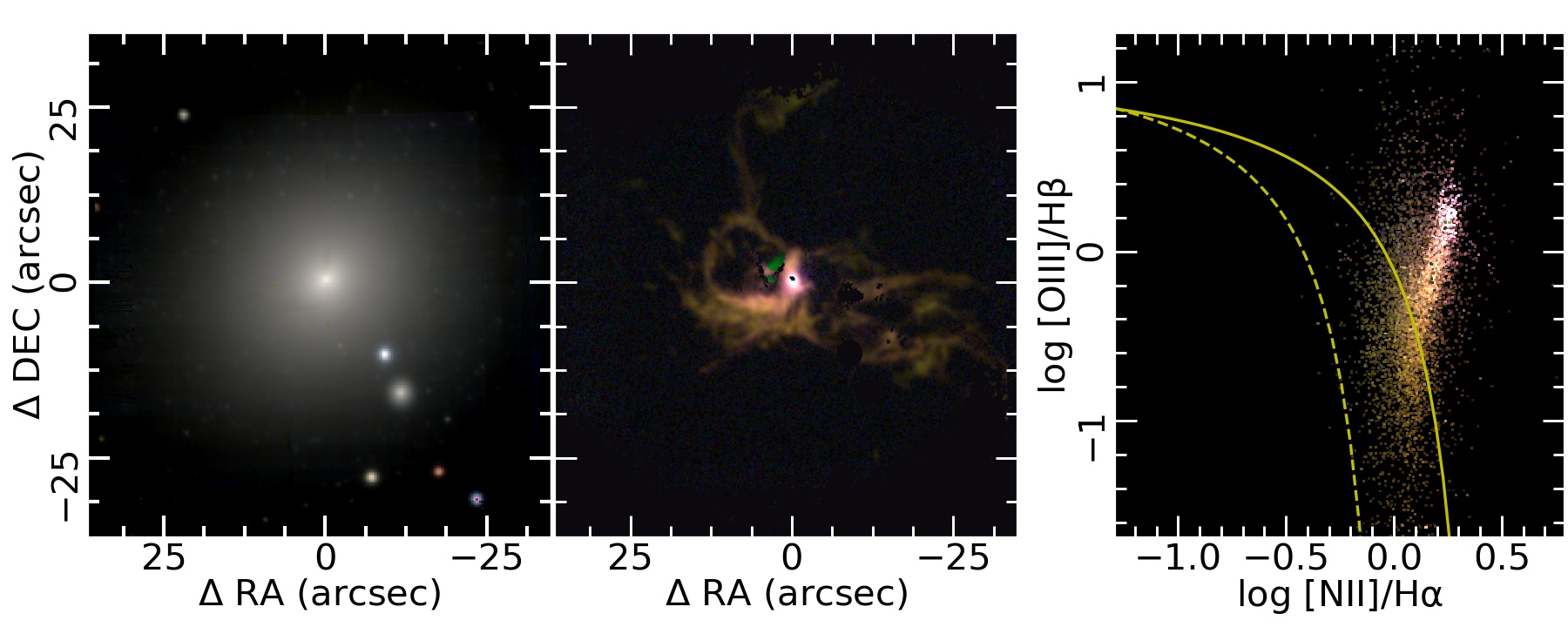
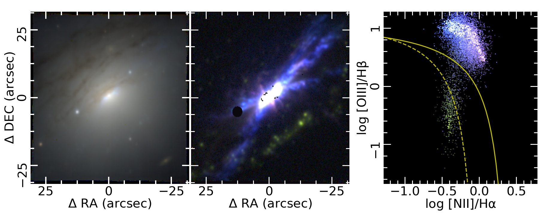
| Figure 4: Color composite continuum and emission line images, and BPT diagram for IC1657 (host of SN2012hd) | |
|---|---|
| original cube: SN2012hd.cube.fits.gz | |
| elimission line information: flux_elines.SN2012hd.cube.fits.gz | |
| Access to the fitsfiles to generate this figure | |
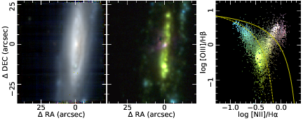 | |
| flux_elines cube is decribed in Sanchez et al. 2016,RMxAA,52,171 |
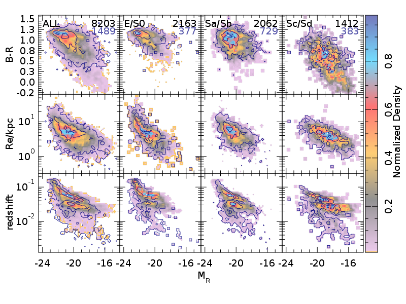
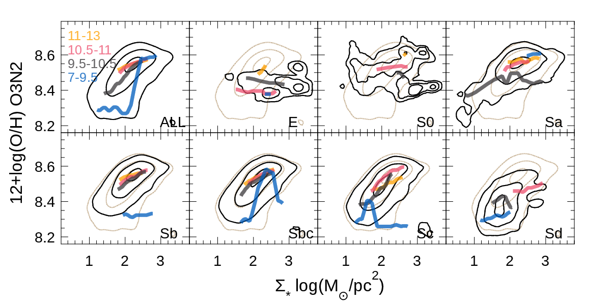
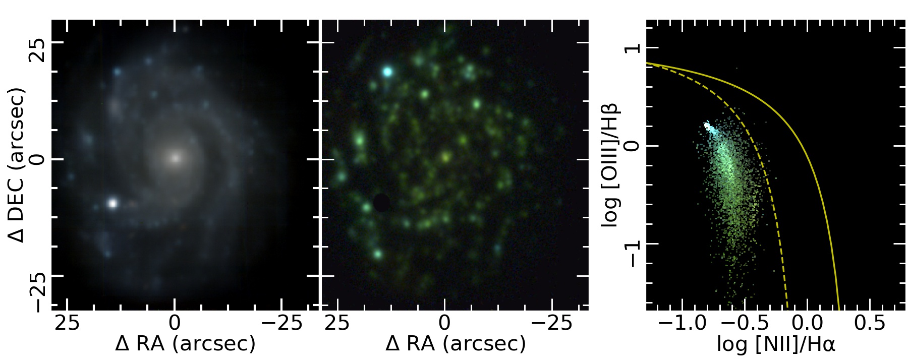
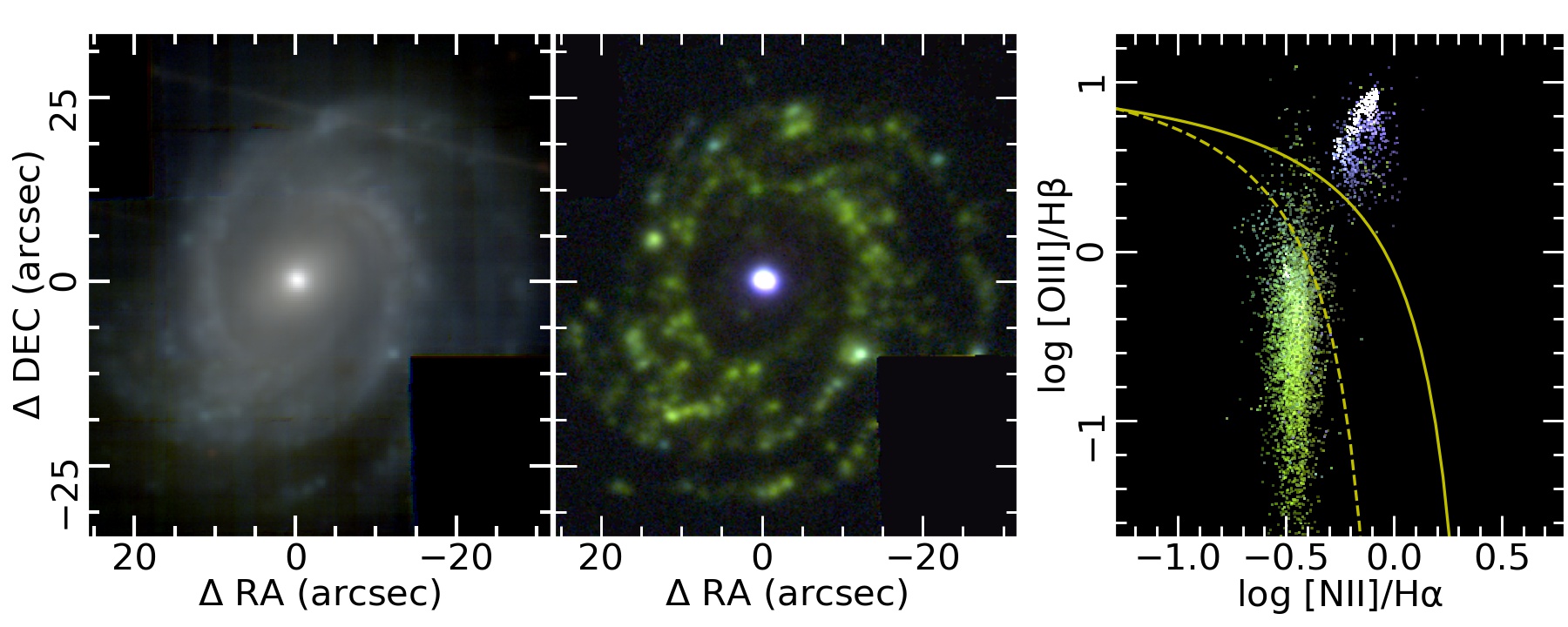
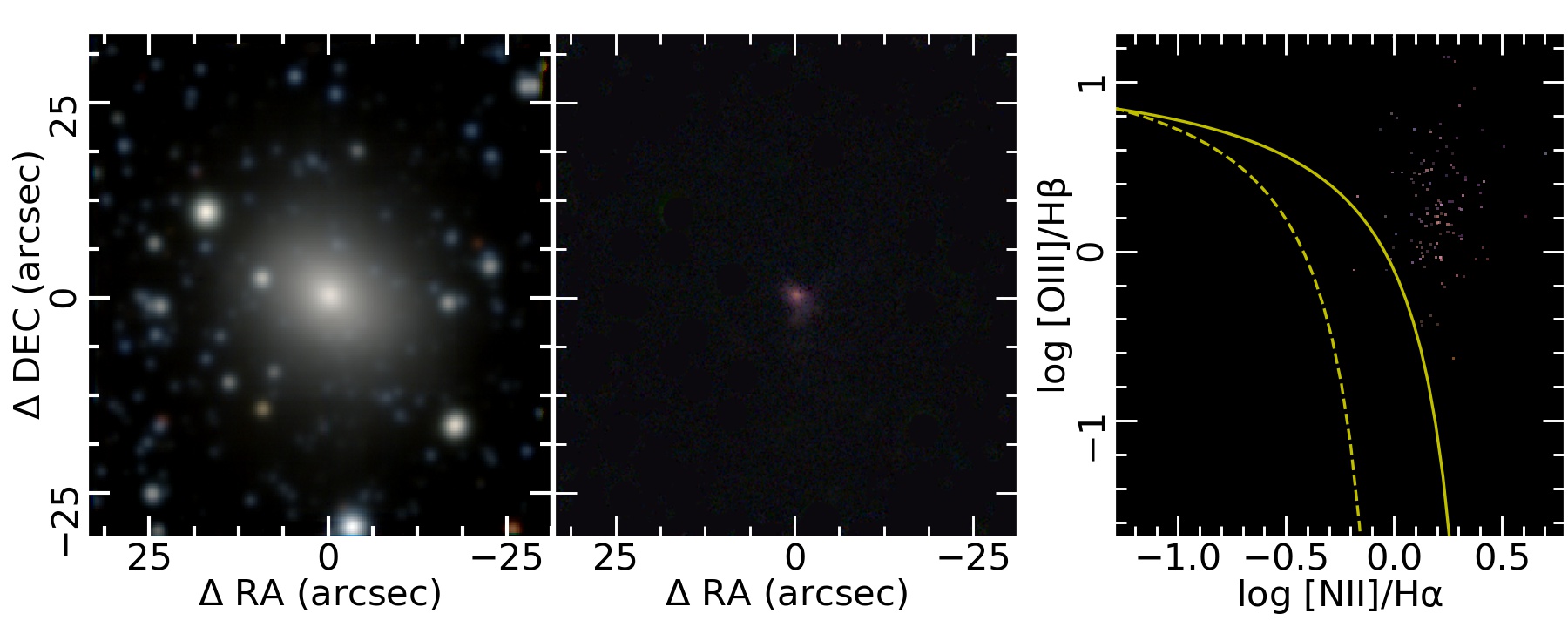
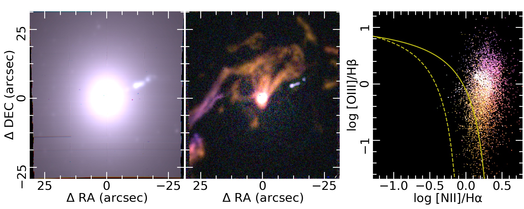
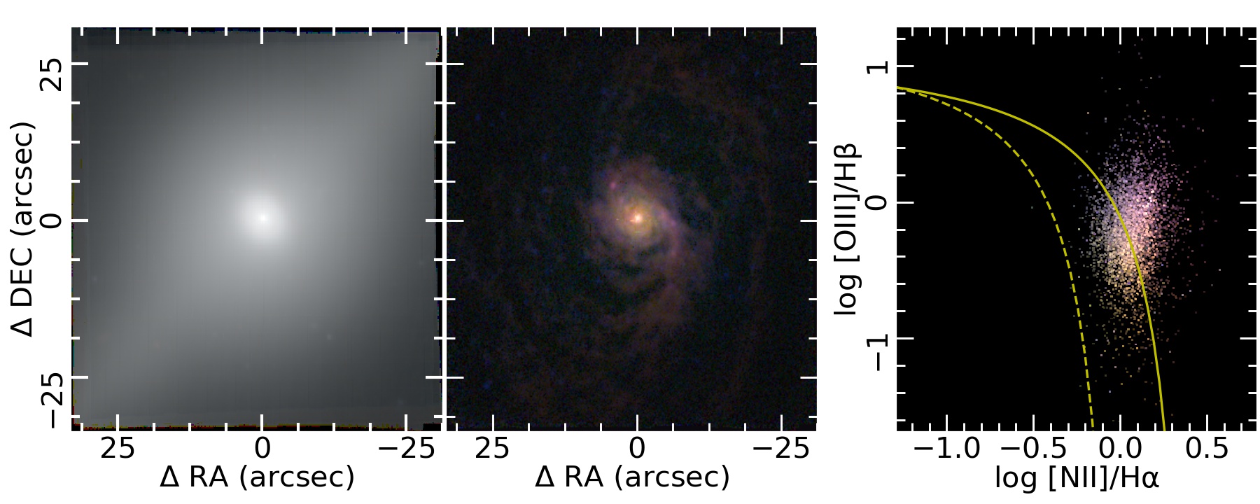
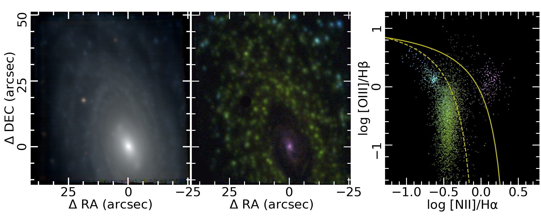
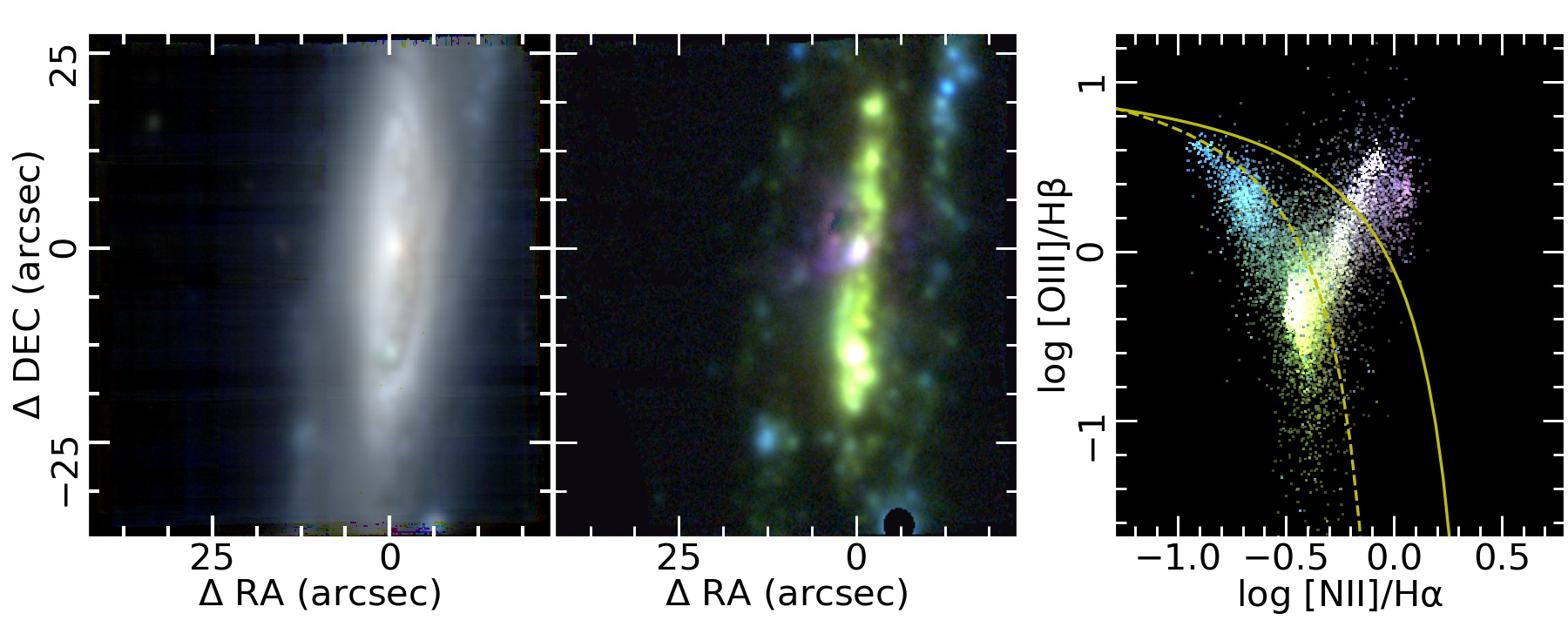
| Figure 5: Spatial resolved BPT diagram | |
|---|---|
| Density maps: SUBSAMPLE.p_e.MAP_diag.fits.gz (contours) | |
| EW maps: SUBSAMPLE.p_e.fMAP_diag.fits.gz (colormaps) | |
| Access to the fitsfiles to generate this figure | |
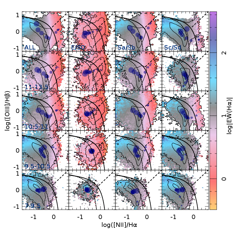 |
SUBSAMPLE describe the subsample of
galaxies included in each panel. E.g.:
ALL for top-left panel |
| The blue dots in the Fig. are included in this table | |
| Figure 6: Spatial resolved Sigma_*-age diagram | |||||||||
|---|---|---|---|---|---|---|---|---|---|
| Density maps: SMass_Age_LW_SUBSAMPLE.p_e.MAP_Mass_Age_LW.fits.gz | |||||||||
| from which the contours are shown in each panel. | |||||||||
| To define the peak density for each mass bin (color lines) it is used the files: | |||||||||
| SMass_Age_LW_SUBSAMPLE_Mass_min_M_max_M.p_e.MAP_Mass_Age_LW.fits.gz | |||||||||
| where min_M and max_M are the min and max stellar mass (logarithmic) of the bin. | |||||||||
| Access to the fitsfiles to generate this figure | |||||||||
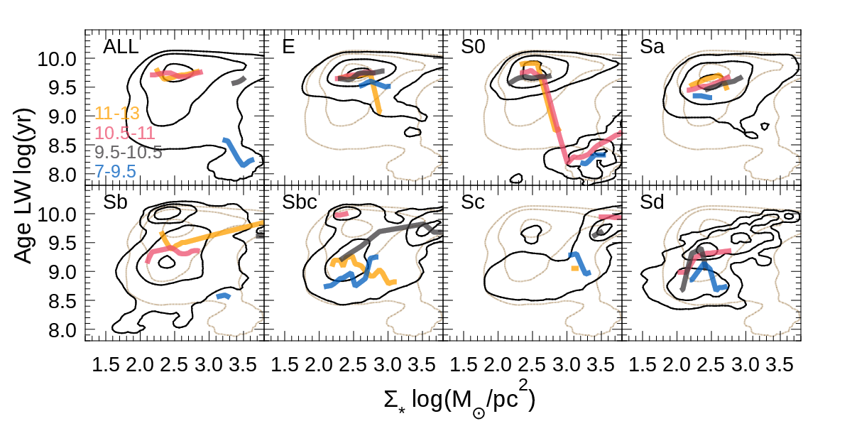 |
SUBSAMPLE describe the galaxy morphologycal type included in each panel, in the following order:
|
||||||||
| E.g., for the 2nd panel there are used the files:
SMass_Age_LW_E.p_e.MAP_Mass_Age_LW.fits.gz (contours) | |||||||||
| Figure 7: Spatial resolved Sigma_*-Sigma_SFR diagram | |||||||||
|---|---|---|---|---|---|---|---|---|---|
| Density maps: SMass_SFR_SUBSAMPLE.p_e.MAP_Mass_SFR.fits.gz | |||||||||
| from which the contours are shown in each panel. | |||||||||
| To define the peak density for each mass bin (color lines) it is used the files: | |||||||||
| SMass_SFR_SUBSAMPLE_Mass_min_M_max_M.p_e.MAP_Mass_SFR.fits.gz | |||||||||
| where min_M and max_M are the min and max stellar mass (logarithmic) of the bin. | |||||||||
| Access to the fitsfiles to generate this figure | |||||||||
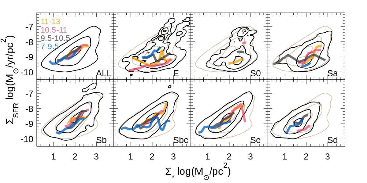 |
SUBSAMPLE describe the galaxy morphologycal type included in each panel, in the following order:
|
||||||||
| E.g., for the 2nd panel there are used the files:
SMass_SFR_E.p_e.MAP_Mass_SFR.fits.gz (contours) | |||||||||
| Figure 8: Spatial resolved Sigma_*-O/H diagram | |||||||||
|---|---|---|---|---|---|---|---|---|---|
| Density maps: SMass_OH_SUBSAMPLE.p_e.MAP_Mass_OH.fits.gz | |||||||||
| from which the contours are shown in each panel. | |||||||||
| To define the peak density for each mass bin (color lines) it is used the files: | |||||||||
| SMass_OH_SUBSAMPLE_Mass_min_M_max_M.p_e.MAP_Mass_OH.fits.gz | |||||||||
| where min_M and max_M are the min and max stellar mass (logarithmic) of the bin. | |||||||||
| Access to the fitsfiles to generate this figure | |||||||||
 |
SUBSAMPLE describe the galaxy morphologycal type included in each panel, in the following order:
|
||||||||
| E.g., for the 2nd panel there are used the files:
SMass_OH_E.p_e.MAP_Mass_OH.fits.gz (contours) | |||||||||
| Figure 10: Spatial resolved Sigma_gas-Sigma_SFR diagram | |||||||||
|---|---|---|---|---|---|---|---|---|---|
| Density maps: SMass_gas_SFR_SUBSAMPLE.p_e.MAP_Mass_gas_SFR.fits.gz | |||||||||
| from which the contours are shown in each panel. | |||||||||
| To define the peak density for each mass bin (color lines) it is used the files: | |||||||||
| SMass_gas_SFR_SUBSAMPLE_Mass_min_M_max_M.p_e.MAP_Mass_gas_SFR.fits.gz | |||||||||
| where min_M and max_M are the min and max stellar mass (logarithmic) of the bin. | |||||||||
| Access to the fitsfiles to generate this figure | |||||||||
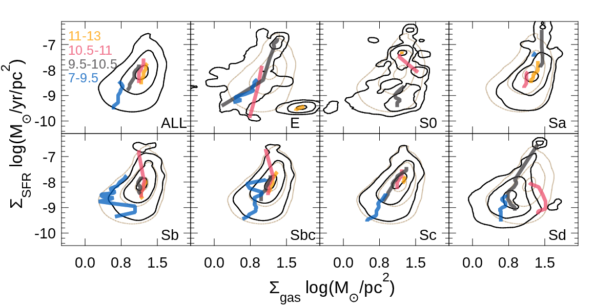 |
SUBSAMPLE describe the galaxy morphologycal type included in each panel, in the following order:
|
||||||||
| E.g., for the 2nd panel there are used the files:
SMass_gas_SFR_E.p_e.MAP_Mass_gas_SFR.fits.gz (contours) | |||||||||
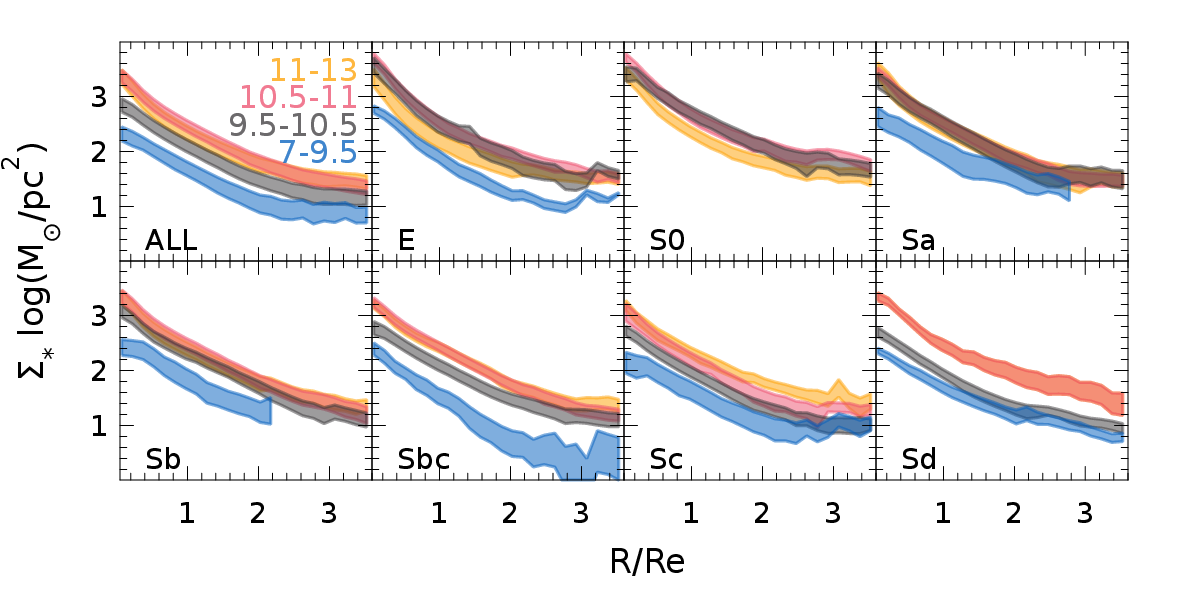
| Figure 11: Distribution of the Sigma_* along the time and radius | |||||||||||||||||||||
|---|---|---|---|---|---|---|---|---|---|---|---|---|---|---|---|---|---|---|---|---|---|
| Radial distribution stored in SUBSAMPLE.p_e.rad_SFH_lum_Mass_C.fits.gz | |||||||||||||||||||||
| Each of these files contains, averaged for each sub-sample, the radial distribution
of Sigma_* (along the Y-axis) for different look-back times (along the X-axis) as recovered from the
stellar population analysis performed by FIT3D. Thus, each vertical cut represents the radial distribution
of Sigma_* at the each considered time, and each horizontal cut represents the growth with time
of Sigma_* at a certain radius. The Y-axis is normalized at the observed (present) effective radius Re, ranging from 0 to 3.5 R/Re, with steps of 0.1 R/Re for each pixel in the Y-axis. The X-axis corresponds ages in logarith scale, starting at log(age/yr)=6.4, and spaning 0.1 dex for each pixel in the X-axis, up to 10.2 dex.
In Fig. 11 we show horizontal cuts average every 5 radial bins for clarity. | |||||||||||||||||||||
| Access to the fitsfiles to generate this figure | |||||||||||||||||||||
 | |||||||||||||||||||||
|
SUBSAMPLE describe the galaxy morphologycal type and mass range in each panel, in the following order:
|
|||||||||||||||||||||
| Figures based on azimutal average radial distributions | |||||||||
|---|---|---|---|---|---|---|---|---|---|
| Figures 9, 12, 13, 14 , 15, 16, 17, 18, 19 are based on the same files: | |||||||||
| SUBSAMPLE_Mass_min_M_max_M.p_e.RAD_ALL.fits.gz | |||||||||
| where min_M and max_M are the min and max stellar mass (logarithmic) of the bin. | |||||||||
| Access to the fitsfiles to generate this figure | |||||||||
| Figure 12 it is shown as an example: | |||||||||
 |
SUBSAMPLE describe the galaxy morphologycal type included in each panel, in the following order:
|
||||||||
| E.g., for the 2nd panel there are used the files:
E_Mass_11_13.5.p_e.RAD_ALL.fits.gz (yellow line) | |||||||||
|
This files (*.p_e.RAD_ALL.fits.gz) are datacubes in which the radial distribution of each
particular property of the galaxies is stored in each slice (or 2D image) along the Z-axis.
The property stored in indicated in a header heyword, named DEC_NN where NN
is the slice index along the Z-axis of the cube, starting with 0. The relevant for this review were: DESC_0 | Stellar mass density in logarithm of Msun/pc^2 (Fig. 12,17) DESC_1 | SFR density in logarith of Msun/pc^2 (Fig. 16,17,19) DESC_2 | Molecular gas mass density derived from Av in log. of Msun/pc^2 (Fig. 18,19) DESC_4 | Lum. Weighted Stellar metallicity [Z/H] (Fig. 9 & Fig. 14) DESC_6 | Lum. Weighted Stellar Ages in log of yr (Fig. 13) DESC_9 | 12+log(O/H) derived using the Marino et al. 2013 O3N2 calibrator (Fig. 16) The remaining parameters in the file were not used in this review, and in some cases are highly experimental. In each slice, the X-axis corresponds to a different galactocentric distance, in units of the effective radius of each galaxy (prior to derive the average by galaxy group). Each pixel corresponds to 0.15 R/Re, ranging from 0 to 3.5Re.
Finally, for each slice, the values at each index in the Y-axis corresponds to:
Y_0 | The galactocentric distance indicated before | |||||||||
| Figure 9: Radial average distribution along the Sigma-[Z/H] diagram | |||||||||
|---|---|---|---|---|---|---|---|---|---|
| It uses the same files as the radial gradients described before. However, in this case it shows the distribution of 2nd row plus/minus the 3rd row of the 5th slice (DESC_4 or NN=4) in the Z-axis along the 2nd raw of the 1st slice (DESC_0 or NN=0), for each cube corresponding to a different subsample. | |||||||||
| Access to the fitsfiles to generate this figure | |||||||||
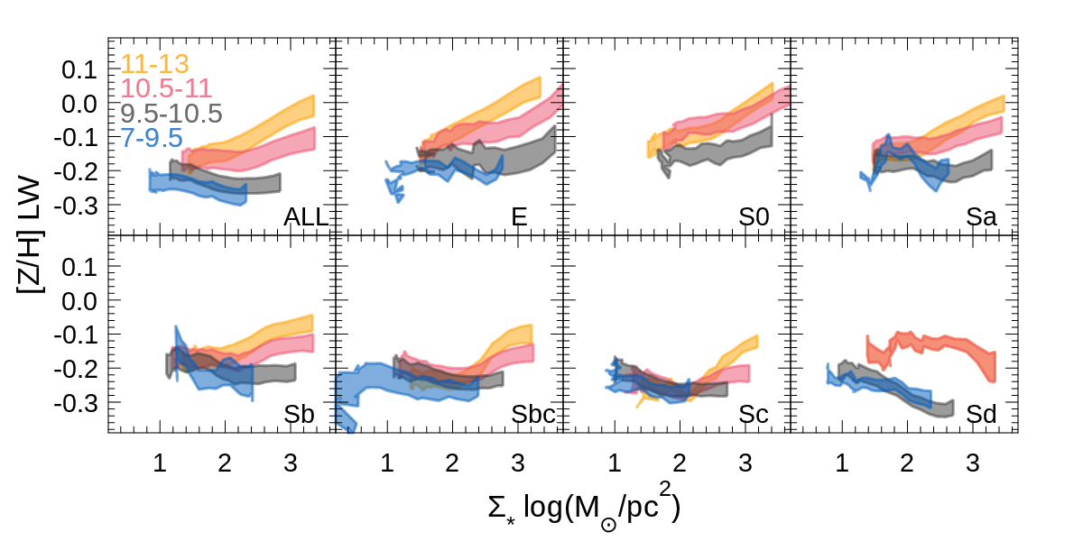 |
SUBSAMPLE describe the galaxy morphologycal type included in each panel, in the following order:
|
||||||||
|